Surface & functions
Navigation
All available reports and settings can be accessed via the navigation bar. Clicking on an entry opens a menu with the selection of the corresponding reports or settings. The layer closes automatically when you click on an entry, by clicking on the close symbol at the top right or by moving the mouse outside the layer. When a report is open, the navigation area in which the report is located is highlighted by a white bar and bold font.
Which functions are available depends on the respective edition. If a function is not available in your edition, a rocket symbol will be displayed behind it to indicate an upgrade option.
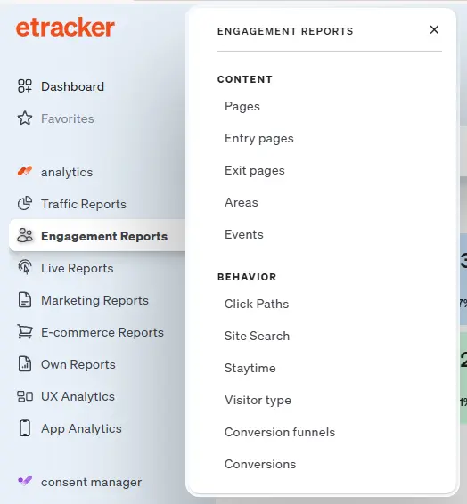
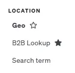
On mouseover, reports can be marked as favorites by clicking on the corresponding star. These reports can then be accessed more quickly.
Introduction to the report interface
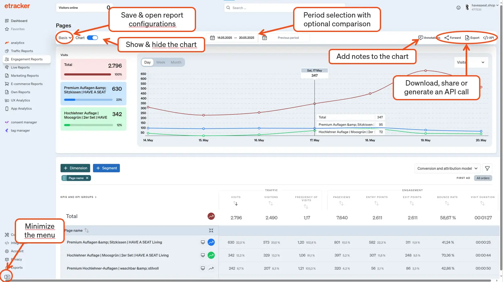
The reports offer the following standard functions:
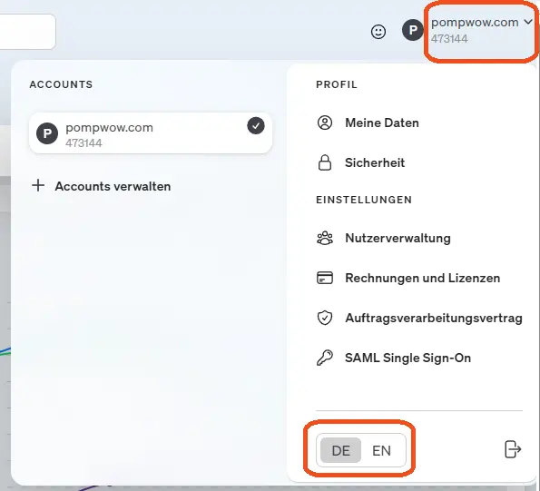
In addition, you can switch between the English and German language versions at any time via the account menu.
Own report configurations (views)
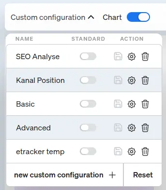
If you frequently make certain settings for a report (period, dimension, segment and/or key figure selection), it makes sense to save these as configurations. You can access the saved configurations via the Custom configuration drop-down menu, saving you time and effort. To save your own configurations, proceed as follows: Select a report and make the desired settings. Click on Custom configuration and in the menu that opens, click on Create new configuration +.
- Define a name for the configuration in the overlay.
- Select the appropriate settings for the configuration:
- Display totals lines: If the configuration is used for further processing in third-party systems, the totals line should be deactivated.
- Share with all users: Share the configuration with all other users if required.
- Use as default: By default, the configuration is loaded directly from the navigation menu when the report is selected.
- Mark as favorite: The configuration can be selected as a favorite directly from the corresponding menu item.
- Click on Save.
You can also change or delete an existing configuration via the configuration menu. You can also click on Reset to return to the standard configuration, i.e. undo all changes made to sorting, filtering, etc.
Period selection
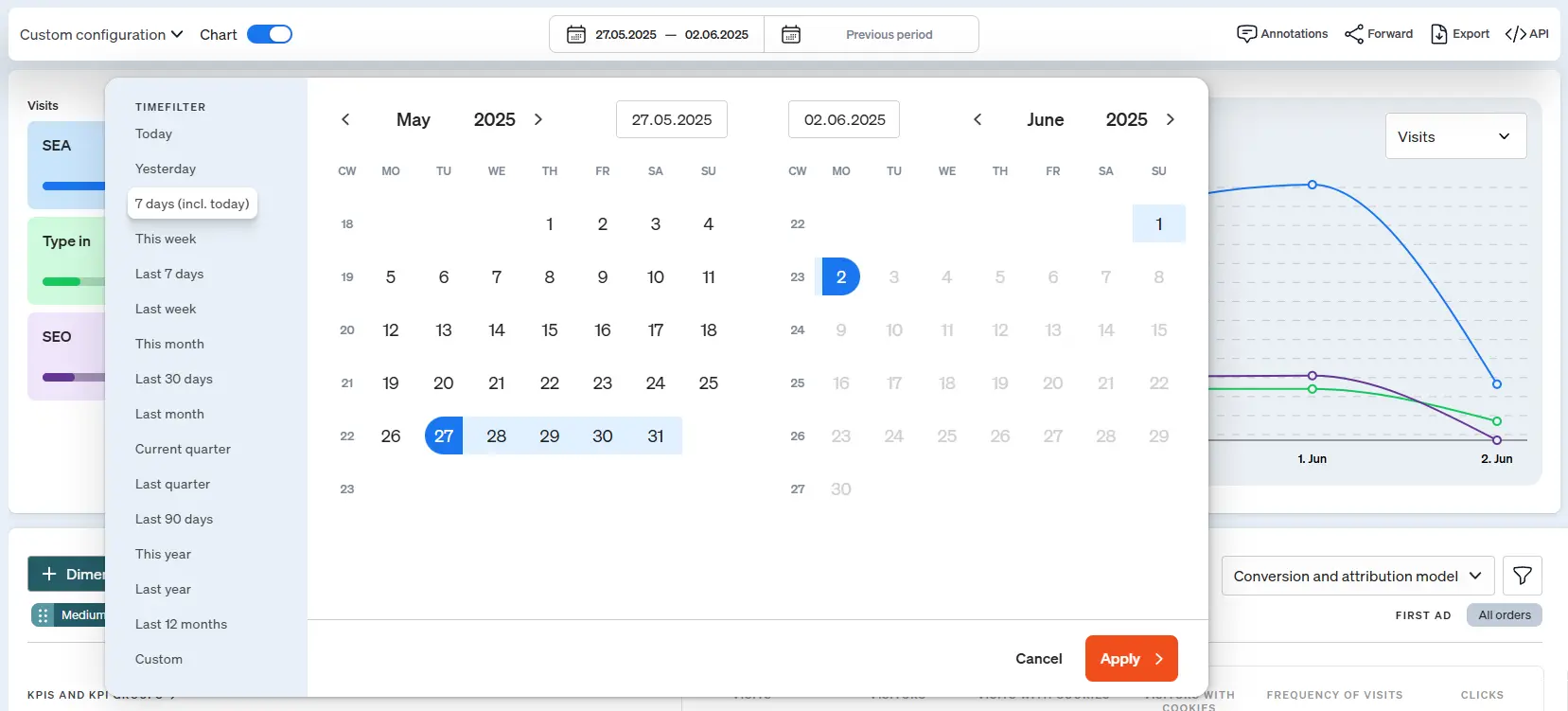
The currently selected period is always displayed in the upper report menu bar. By default, the evaluation period covers the last seven days including the current day. Clicking on the period button opens the calendar to adjust the evaluation period. Predefined periods can be selected in the calendar selection list for quick period settings (e.g. Current week, Current month).
Notes
It is possible to add notes to each report in order to record the background of changes.

The note function is located in the top bar of each report:

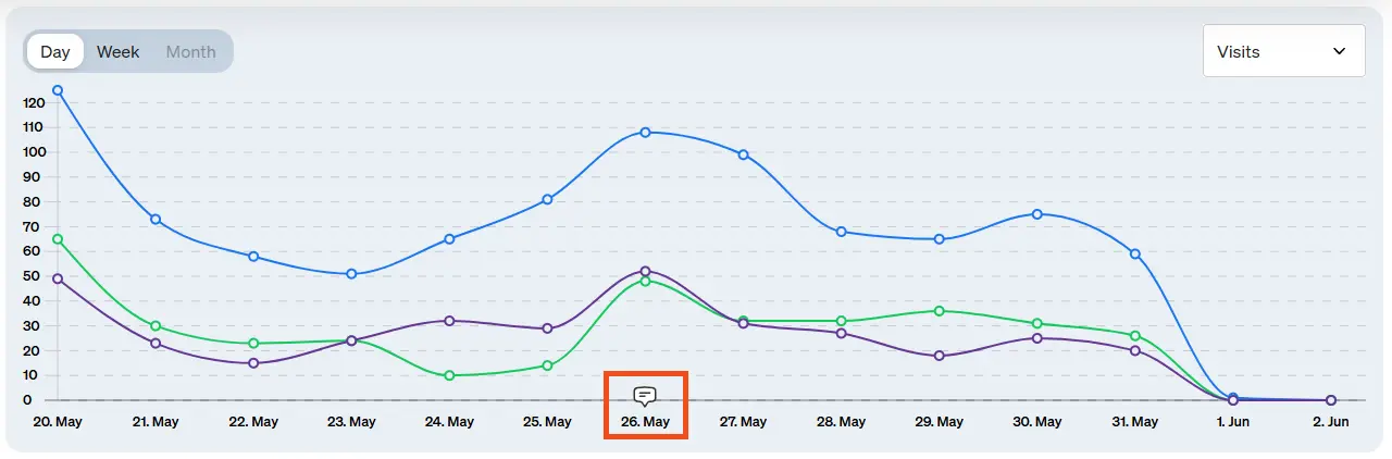
There you can see directly whether notes are available in the set period. If notes are available, the speech bubble appears with the number of notes. The notes can be displayed and edited by clicking on the speech bubble or the menu item:
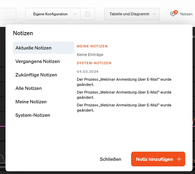
There are two types of notes: your own notes and system notes. The system notes are created automatically if, for example, a conversion process has been edited. You can create your own notes via Add note.
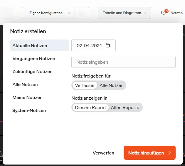
Here you can set the associated date and specify who should view this note and whether this note should be displayed in a specific report or in all reports.
Notes are also displayed in the graphic on the timeline using a speech bubble and can be opened via mouse-over:
Exporting, forwarding and processing reports
To download individual report data, select the export function at the top right of the report menu. The formats CSV, XML, XML (Excel), XLS, PDF and export.json are available for selection. If the report is to be exported regularly or recurrently with certain settings, use the automated e-mail reporting.
The report data can be forwarded in a similar form via email attachment. When using the Enterprise Edition, the corresponding API call can be generated and used for the selected report configuration.
Diagram
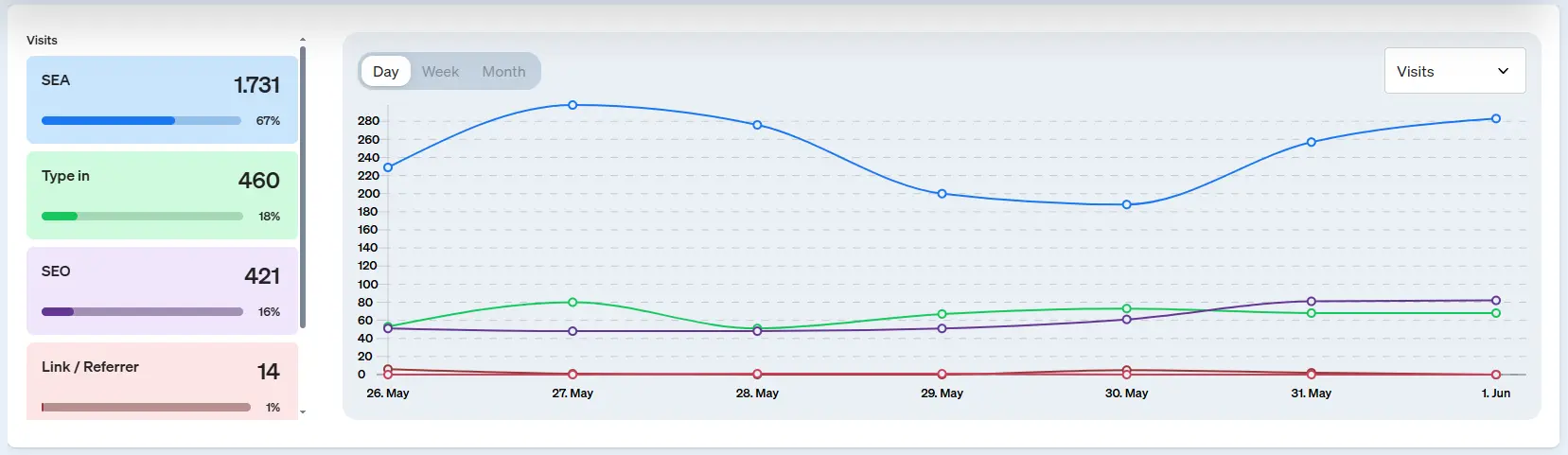
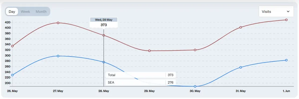
The chart visualizes the values of the table over time. The tiles on the left show the total values and percentages of the selected entries and at the same time the corresponding colors of the lines in the chart. The entries for the chart can be selected and deselected using the buttons in the dimensions column.
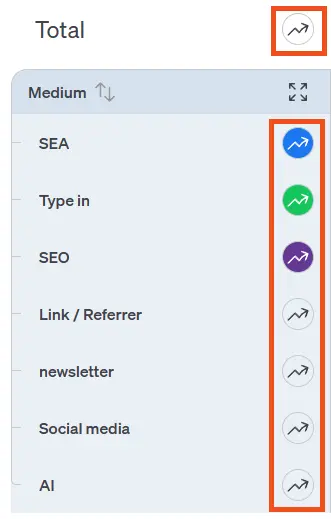
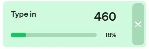
Diagram entries can also be removed via the tile bar by moving the mouse pointer over them and clicking on the X.
If you move the mouse pointer along the time axis, the values for each line at the respective point in time appear.
The following options are available for adjusting the diagram:
- Select key figure: Use the key figure button at the top right of the graphic to select the key figure from the key figures available for the table.
- Change interval: In addition to daily changes, you can also select monthly or weekly intervals for longer periods.
Table
The tabular view offers a variety of functions for deriving findings.
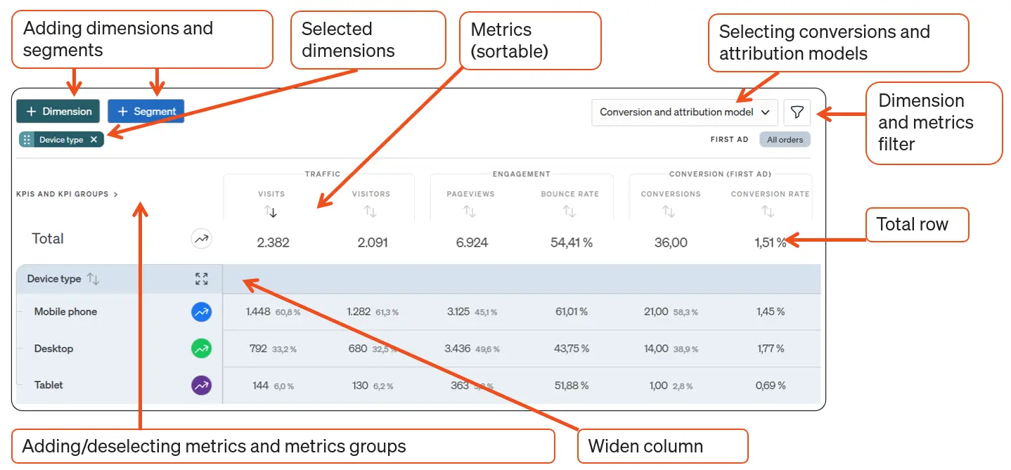
The evaluation functions include
Segmentation
You can use + Segment to select or configure your own behavioral segments with corresponding conditions.
Dimensions
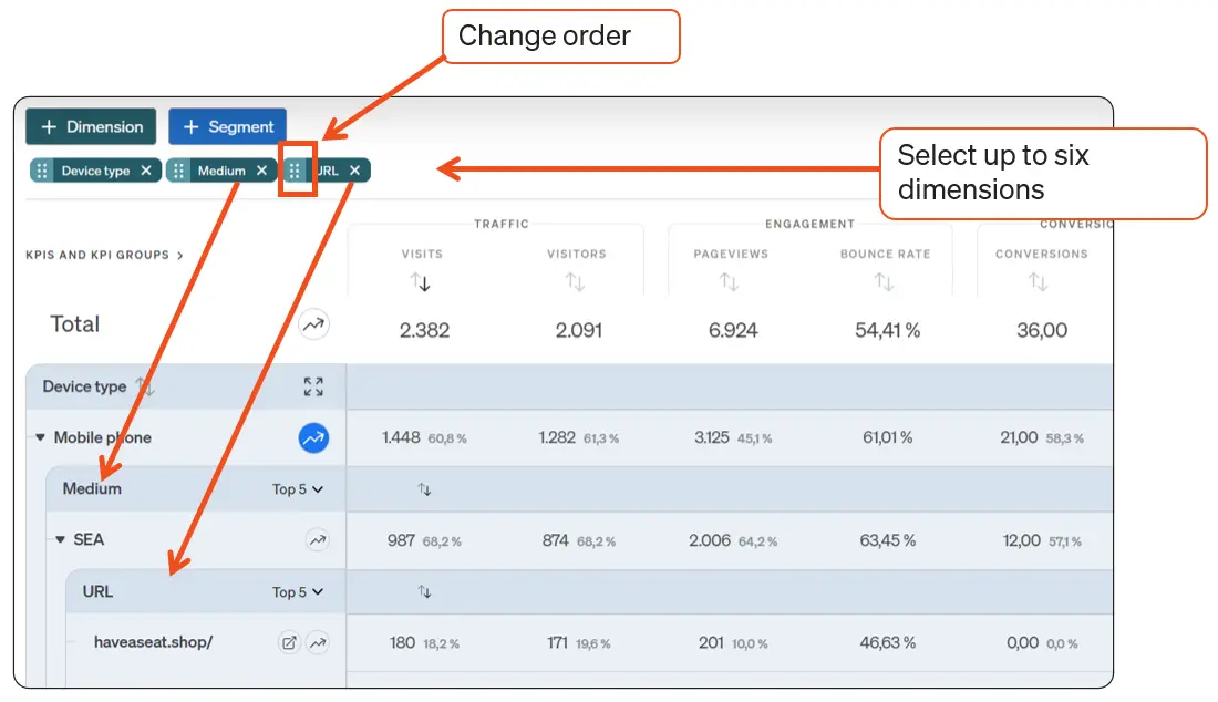
The analysis of the data can be broken down further using +Dimension. The dimension selection does not simply set a filter and reduce the data, but rather enables a complete drill-down to all dimension values. By default, the top 5 dimension values are displayed in the table for the top dimension when you click on the arrow to the right of an entry. You can extend the number of entries displayed up to the top 100 values. You can undo the drill-down for each entry in the same way by clicking on the arrow pointing downwards.
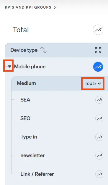
etracker analytics enables multi-dimensional drill-down in a very dynamic form. This allows you to explore the interplay of different dimensions. You also have the option of changing the order of the dimensions by moving the handle of the respective dimension in the dimension bar.
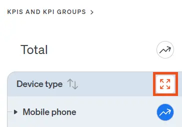
Increase dimension column width
The arrows in the top right-hand corner of the dimensions column can be used to increase or decrease the width in order to display more characters.
Sort key figures
The values of the key figures can be sorted in ascending or descending order by clicking on a column heading . The current sort criterion is indicated by the highlighted sort arrow below the respective key figure name.
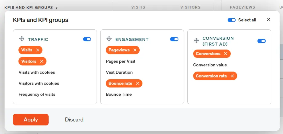
Show/hide and re-sort key figures
To show or hide key figures or key figure groups, click on the corresponding entry on the left above the dimensions column. In the dialog that opens, individual key figures within the groups or entire key figure groups can be selected or deselected. The sorting of the key figure groups can also be changed using the handles at the top left of the group boxes. Then click on Done to apply the settings.
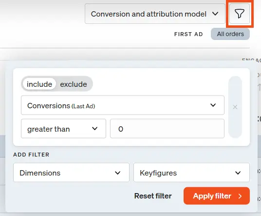
Filter attributes and key figures
The reports can be filtered according to specific dimension values and key figure values. The filter function is located on the right above the table. The filter can be configured in the upper area or removed using the delete button on the right. New filter conditions can be added for dimensions or key figures. Several filter conditions can be combined.
Selection of conversions and attribution model
Switch between different conversion attribution models with a single click. The switch is located on the right above the table. The menu that opens can also be used to change the selection of conversions to be taken into account.
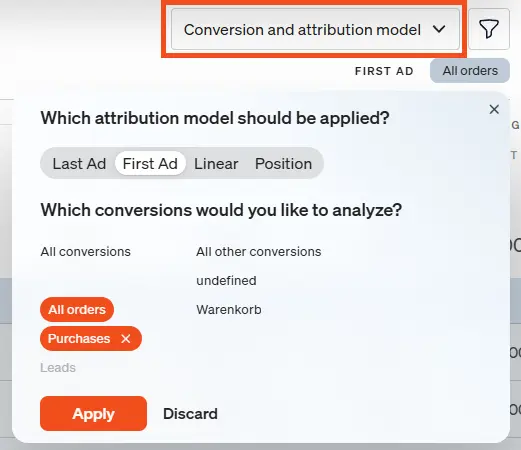
Available distribution models:
- Last Ad (standard model): The conversion is assigned to the last entry source.
- First Ad: The conversion is assigned to the first entry source.
- Linear (equal distribution): The conversion is evenly distributed between all entry sources. All touchpoints receive the same share or the same rating.
- position (also known as the bathtub model): Conversion is assigned to the first and last contact with 40% each and the rest with 20%. The first and last entry sources therefore each receive the highest value.
Type-ins are only included in the evaluation if the contact chains (see Marketing Reports → Contact combinations) only contain the type-in medium.
Period comparison
The period comparison allows you to compare data from a more recent period with data from an older period. The changes are also visualized with coloured arrows so that you can see at a glance which key figures have changed positively or negatively. Please note that the comparison is only visualized in the report table. The data for the selected period continues to be displayed in the diagram.
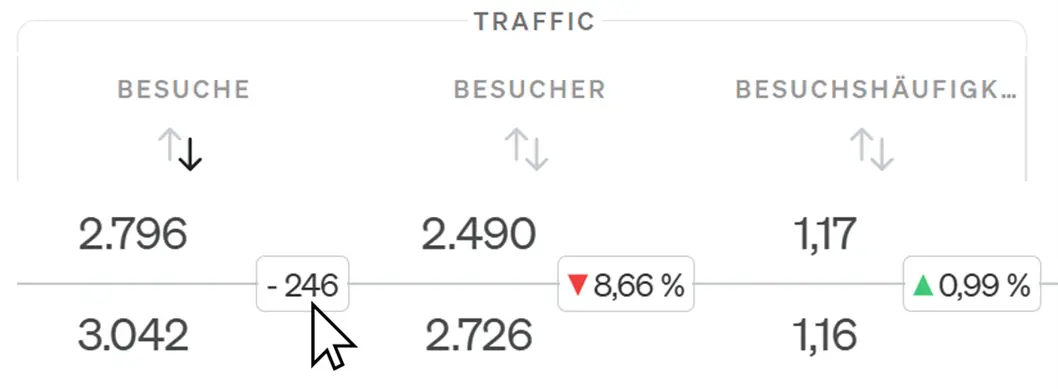
The current values are displayed for each entry, the past values below them and the percentage changes between them on the right. The deviation is also shown by a green arrow pointing upwards (better than in the comparison period) or a red arrow pointing downwards (worse than in the comparison period). On mouseover, the percentage display changes to an absolute display of the change.
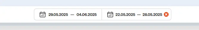
The red X next to the display of the comparison period in the report can be used to end the period comparison.